Ptychography analysis using a command-line script

The simplest way to analyse a ptychography dataset using PyNX is to use a command-line script.

Note regarding command-line arguments:

• previous versions of PyNX (<2024) used e.g. pynx-ptycho-cxi data=data.cxi

• now command-line arguments all start with -- to use standard parsing libarries and make it easier to documentation

• you can use equivalently pynx-ptycho-cxi --data=data.cxi or pynx-ptycho-cxi --data data.cxi, with the exception of options where the supplied value begins with --, e.g. it is mandatory to use --defocus=-200e-6, as using --defocus -200e-6 will try to interpret -200e-6 as a new command-line argument

The generic pynx-ptycho-cxi script reads data from a CXI file (see http://cxidb.org, see below how to create such a file) including data for a two-dimensional projection. A simple data analysis can be done using:

pynx-ptycho-cxi --data=data.cxi --probe=gaussian,200e-9x200e-9 --liveplot --saveplot
                --algorithm=analysis,ML**100,DM**200,nbprobe=3,probe=1``

This will import the data from the data.cxi, which includes all information (observed frames, motor positions, detector distance, wavelength, mask…), and then optimise the object and probe.

The algorithm string is interpreted right-to-left (without any space):

• probe=1 activates the probe optimisation (by default only the object is optimised)

• nbprobe=3 activates 3 probe modes

• ML**100,DM**200: run 200 cycles of Difference Map, followed by 100 cycles of conjugate gradient Maximum Likelihood.

• analysis: analyse the final probe, determining the position of the focus and plotting it, and the probe modes.

The initial shape for the probe (probe=gaussian,200e-9x200e-9) will be a Gaussian with a horizontal x vertical width of 200 x 200 nm**2.

The liveplot and saveplot keywords will trigger the display of plots during the optimisation (Note that unless the dataset is quite large, this will significantly slow down the optimisation), and the saving of the final object and probe.

All results (CXI output and plots) are saved in a subdirectory ResultsScanNNNN, where NNNN is the scan number.

You can try this using an example dataset. On a Linux or macOS computer:

# If necessary, activate your python environment with PyNX
source /path/to/my/python/environment/bin activate

# Download example dataset
curl -O http://ftp.esrf.fr/pub/scisoft/PyNX/data/ptycho-siemens-star-id01.cxi

# View the CXI file using the silx viewer:
silx view ptycho-siemens-star-id01.cxi

# Run the PyNX analysis script
pynx-ptycho-cxi --data ptycho-siemens-star-id01.cxi --liveplot saveplot\
                --algorithm=analysis,ML**100,DM**200,nbprobe=3,probe=1 \
                --probe=focus,60e-6x200e-6,0.09 --defocus=200e-6

# View the result from the output CXI file using the silx viewer
silx view ResultsScan0013/latest.cxi

# You can also open latest.png, latest-probe-modes.png and
latest-probe-z.png in ResultsScan0013.

In this script, the initial probe is simulated from a 60x200 microns aperture, focused 9 cm, and then defocused 200 microns

Example output images (click on images for a larger view):

Object and probe plot

Probe focus analysis

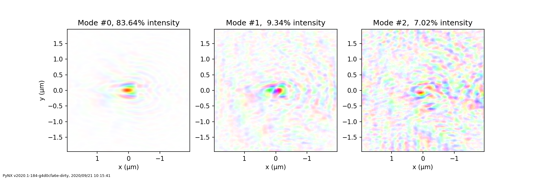
Probe modes analysis

Important note

Getting a correct result during ptychography analysis can be fairly easy if you are looking at a good dataset, with a structured probe, a varied object and enough statistics in the experimental data. However there are many cases where the data is more ill-configured. In which case there are a number of options which should be considered, such as the object and probe inertia and/or smoothing, the position optimisation, etc…

Similarly the starting object and probe can be important: in the example dataset above, the diversity of the scattering from the siemens star, recorded with good statistics, allows convergence starting far from the solution. In other cases, it is important to start from relatively good defaults in order to speed up the convergence, e.g. using a probe from a previous optimisation. Also, at high energy, starting from a phase object (amplitude near 1 and a given phase range) can help the converegence.

In some cases if the algorithms tend to be unstable, it is possible to rely on the alternating projections (AP) algorithm, which is fairly stable even if much more slowly converging than DM.

More information

The full documentation for the command-line scripts can be obtained by using the --help command-line option, e.g.:

pynx-ptycho-cxi --help

For more information, please read the online documentation on Ptychography scripts

Creating a CXI file

To create a CXI file from data (see http://cxidb.org), the save_ptycho_data_cxi() function can be used:

from pynx.ptycho import save_ptycho_data_cxi
save_ptycho_data_cxi(file_name, iobs, pixel_size, wavelength, detector_distance, x, y)

See the corresponding API documentation at: pynx.ptycho.ptycho.save_ptycho_data_cxi()

Note that it is critical to get the motor and detector orientation right. The detector origin should be at the top, left corner, as seen from the sample. The X sample position coordinate should be horizontal, towards the left as seen from the X-ray source, and the Y coordinate should be vertical, looking towards the ceiling. This corresponds to the CXI convention (see http://cxidb.org), itself deriving from the NeXus and McStas ones.

To test all possible orientations (motor and image axes orientation and exchange), you can also try to use the --orientation_round_robin command-line keyword, which will test a grand total of 64 possibilities (a number being equivalent), with 8 motor axes and 8 image flip/transpose combinations. This can be unstable, so using a stable algorithm such as AP**1000 is recommended. This approach works best with a standard target such as a Siemens star. It takes a little while, as all possible motor and detector orientations are tested (64 in total), and many are equivalent.